ECE 544 Pattern Recognition¶

约 6575 个字 17 行代码 7 张图片预计阅读时间 22 分钟

Pattern Recognition¶

Pattern recoginition

input data: x
Label/output: y
x^(i)^ -> model/algorithm -> y^(i)^ ---inference/prediction
y=y^(k)^ where k= arg min || x(i)-x||^2=argmin d(x(i)-x)

argmin (argument of the minimum) finds the input value(s) that produce the minimum output of a function, rather than the minimum output itself

K Nearest Neighbor

Linear Regression¶

线性回归

norm

transpose

Expectation: $E_{p(y)[f(y)]}=\sum_{y_i}p(y)f(y)$

arg min

Model: y=w_1\times x+w_2

Error: vertical lines

Set the derivative to zero

Regularization

\[\mathbf{X}\mathbf{X}^T \mathbf{w} + C\mathbf{w} - \mathbf{X}\mathbf{Y} = 0\]

w ∗ = XX ⊤ + CI −1 XY

Higher Po

Maximize the likelihood of the given dataset $D = \{(x(i) , y(i) )\}$ assuming

samples to be drawn independently from an identical distribution

(i.i.d.).

IID? independent identical d

Joint distribution = product of individual distributions

not good for classification

Logistic Regression¶

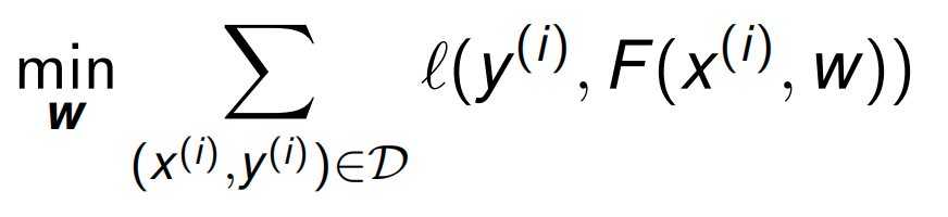
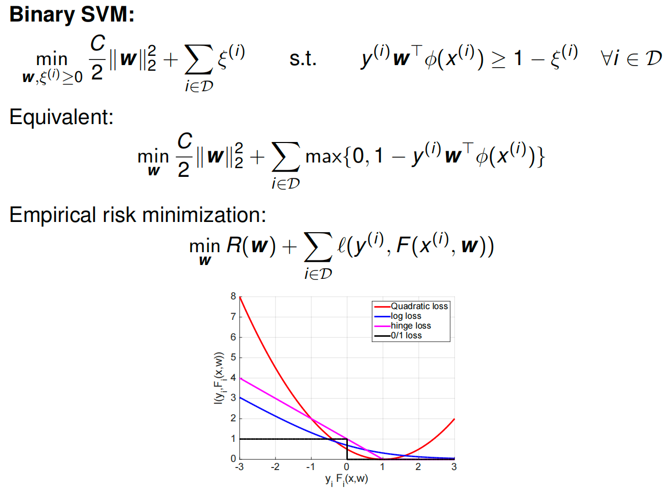
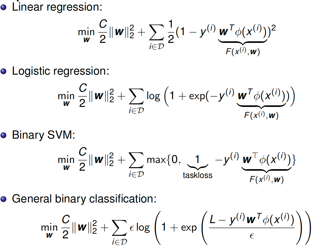
empirical risk minimization

Log(1)

Edge/Boundary detection

[!NOTE]

Which loss is used for logistic regression?

What is the difference between logistic and linear regression?

How to optimize linear and logistic regression?

Optimization Primal¶

When can we find the optimum?

Least squares, linear, and convex programs can be solved

efficiently and reliably

Convex set: A set is convex if for any two points w1, w2 in the set, the line segment $λw_1 + (1 − λ)w_2$ for λ ∈ [0, 1] also lies in the set.

Convex function A function f is convex if its domain is a convex set, and for any points w1, w2 in the domain and any λ ∈ [0, 1] $f((1 − λ)w1 + λw2) ≤ (1 − λ)f(w1) + λf(w2)$

Show that $log(1 + e^x)$ is convex for x ∈ R

convex optimization

Gradient descent

[!NOTE]

Stepsize/Learning rate rules?

Descent directions?

Properties of convex functions?

Convergence rates?

Improvements?

Important topics of this lecture

Convex optimization basics

Algorithm choices

Rates

Optimization Dual¶

Lagrangian

Recipe for computing dual program:

Bring primal program into standard form
Assign Lagrange multipliers to a suitable set of constraints
Subsume all other constrains in W
Write down the Lagrangian L
Minimize Lagrangian w.r.t. primal variables s.t. w ∈ W

Karush-Kuhn-Tucker (KKT) conditions

The Relationship: Primal vs. Dual

The relationship is built on the inequality you saw earlier:

\[\min_{\mathbf{w}} L(\mathbf{w}, \lambda) \le f_0(\mathbf{w}^*)\]

The Primal Program minimizes the cost directly (finding the lowest valley).
The Dual Function $g(\lambda)$ finds a lower bound for that cost (finding the highest possible "floor" beneath the valley).
The Dual Program is simply the search for the best (highest) lower bound. It asks: "What is the largest possible value for this floor?"

Walkthrough: The Linear Program Example

Let's trace the steps in the slide to see how we get from the Primal to the Dual.

Step 1: The Primal Problem

We start with a standard linear minimization:

\[\min_{\mathbf{w}} \mathbf{c}^T \mathbf{w} \quad \text{s.t.} \quad \mathbf{A}\mathbf{w} \le \mathbf{b}\]

Step 2: The Lagrangian

We add the constraint to the objective using a Lagrange multiplier $\lambda$ (where $\lambda \ge 0$).

\[L(\mathbf{w}, \lambda) = \mathbf{c}^T \mathbf{w} + \lambda^T (\mathbf{A}\mathbf{w} - \mathbf{b})\]

Step 3: Regroup terms by $\mathbf{w}$

To find the minimum with respect to $\mathbf{w}$, we need to group all terms containing $\mathbf{w}$ together.

\[L(\mathbf{w}, \lambda) = (\mathbf{c} + \mathbf{A}^T \lambda)^T \mathbf{w} - \mathbf{b}^T \lambda\]

Here, $(\mathbf{c} + \mathbf{A}^T \lambda)$ acts like the slope of a line.
$-\mathbf{b}^T \lambda$ acts like the intercept (constant with respect to $\mathbf{w}$).

Step 4: Minimize $L$ to find $g(\lambda)$

We need to find $\min_{\mathbf{w}} L(\mathbf{w}, \lambda)$. This is the tricky part shown in the middle of the slide.

Think of this as minimizing a simple line $y = mx + b$.

Case A: If the slope $m$ is not zero (i.e., $\mathbf{c} + \mathbf{A}^T \lambda \neq 0$), we can choose $\mathbf{w}$ to be huge and negative (or positive), making the total value go to $-\infty$.
Case B: If the slope $m$ is zero (i.e., $\mathbf{c} + \mathbf{A}^T \lambda = 0$), the $\mathbf{w}$ term disappears completely. The value is just the intercept: $-\mathbf{b}^T \lambda$.

So, the dual function $g(\lambda)$ is:

\[g(\lambda) = \begin{cases} -\mathbf{b}^T \lambda & \text{if } \mathbf{A}^T \lambda + \mathbf{c} = 0 \\ -\infty & \text{otherwise} \end{cases}\]

Step 5: The Dual Program

The Dual Program tries to maximize $g(\lambda)$.

Since we want to maximize something, we can ignore the case where it equals $-\infty$ (that's definitely not the maximum!). We only care about the case where the slope is zero.

Thus, the Dual Program becomes:

\[\max_{\lambda \ge 0} -\mathbf{b}^T \lambda \quad \text{subject to} \quad \mathbf{A}^T \lambda + \mathbf{c} = 0\]

Summary

The Lagrangian allowed us to convert a minimization problem over $\mathbf{w}$ (Primal) into a maximization problem over $\lambda$ (Dual).

Primal: Constraints were on $\mathbf{w}$ ($\mathbf{Aw} \le \mathbf{b}$).
Dual: Constraints are on the "slope" being zero ($\mathbf{A}^T \lambda + \mathbf{c} = 0$).

[!NOTE]

What to do before computing the Lagrangian?

How to obtain the dual program?

Why duality

Support Vector Machines¶

SVMs

SVM: Finds the optimal line (hyperplane) that separates the classes with the maximum margin.

\[y_i(\mathbf{w}^T \mathbf{x}_i + b) \ge 1\]

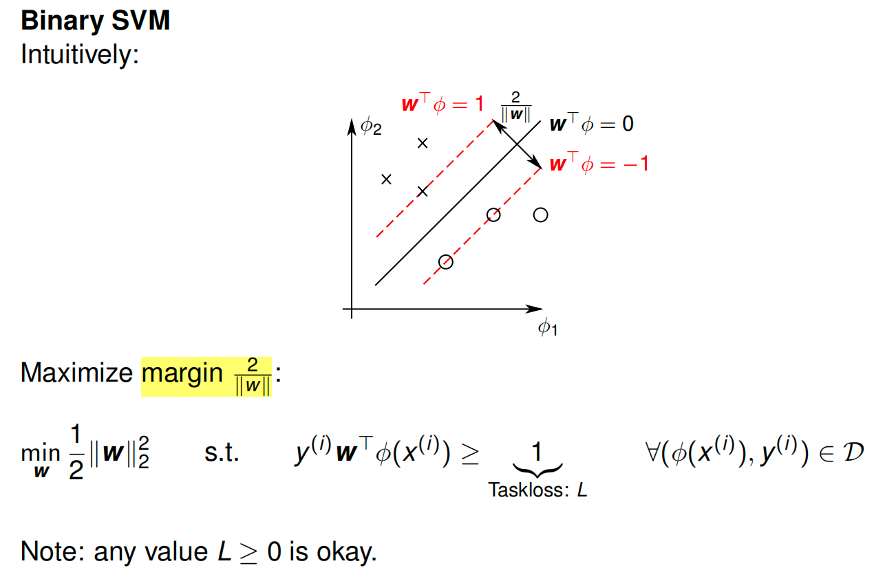
The graph shows data points from two classes (crosses $\times$ and circles $\circ$) in a 2D feature space ($\phi_1, \phi_2$).

The Solid Line ($\mathbf{w}^T \phi = 0$): This is the Decision Boundary. It effectively separates the two classes.
The Dashed Lines ($\mathbf{w}^T \phi = 1$ and $-1$): These represent the edges of the "street" (or margin). The SVM requires all data points to be outside these lines.
The Support Vectors: Notice that only a few points (two crosses and one circle) actually touch the dashed lines. These are the "Support Vectors" that define the model.
The Margin Width ($\frac{2}{\|\mathbf{w}\|}$): The diagram labels the distance between the two dashed lines as $\frac{2}{\|\mathbf{w}\|}$. This is the "safety gap" between the classes.

The Mathematical Goal

The goal of SVM is to make this safety gap (margin) as wide as possible.

Maximize Margin: We want to maximize $\frac{2}{\|\mathbf{w}\|}$.
Minimize Norm: Mathematically, maximizing $\frac{2}{\|\mathbf{w}\|}$ is the same as minimizing $\|\mathbf{w}\|$ (the length of the weight vector).
The Formula: To make the calculus easier, we square it and add a fraction. So, the objective becomes:

\[\min_{\mathbf{w}} \frac{1}{2} \|\mathbf{w}\|_2^2\]

This is what you see in the "Maximize margin" section of the slide.

The Constraints (The Rules)

We can't just minimize $\|\mathbf{w}\|$ to zero (which would make the margin infinite but classify nothing). We must respect the data.

\[y^{(i)} \mathbf{w}^T \phi(x^{(i)}) \ge 1\]

This inequality (labeled "Taskloss: $L$") enforces two things:

Correct Classification: The prediction must have the same sign as the label $y$.
Safety Distance: The prediction value must be at least 1 (or $-1$). This ensures points don't just "barely" cross the line, but stay completely off the "street."

[!NOTE]

"Issue: what if data not linearly separable?".

The model shown here (Hard Margin SVM) crashes if you have a single data point in the wrong crowd (e.g., a blue circle in the middle of the black crosses).

This hints at the next topic in your course: Soft Margin SVM, which introduces "slack variables" to allow for some errors.

Slack

Maximum and constraints

Dual variables $α (i) ≥ 0$ for each inequality constraint

Step 1: Minimize w.r.t. the Weights ($\mathbf{w}$) 第一步：减少权重 $\mathbf{w}$

We want to find the $\mathbf{w}$ that minimizes $L$. We take the derivative with respect to $\mathbf{w}$ and set it to zero. 我们想找到 $\mathbf{w}$ 使 $L$ 最小化的。我们取导数， $\mathbf{w}$ 并将其设为零。

Lagrangian terms with $\mathbf{w}$: $\frac{C}{2}\|\mathbf{w}\|_2^2 - \mathbf{w}^T \sum_i \alpha^{(i)} y^{(i)} \phi(x^{(i)})$ 拉格朗日项为 $\mathbf{w}$ ： $\frac{C}{2}\|\mathbf{w}\|_2^2 - \mathbf{w}^T \sum_i \alpha^{(i)} y^{(i)} \phi(x^{(i)})$
Derivative: 衍生品：

\[\frac{\partial L}{\partial \mathbf{w}} = C\mathbf{w} - \sum_{i} \alpha^{(i)} y^{(i)} \phi(x^{(i)}) = 0\]
Result (Solution for $\mathbf{w}$): 结果（解）： $\mathbf{w}$

\[\mathbf{w} = \frac{1}{C} \sum_{i} \alpha^{(i)} y^{(i)} \phi(x^{(i)})\]

(This tells us that the weight vector is just a linear combination of the data points.) （这告诉我们权重矢量只是数据点的线性组合。）

Step 2: Minimize w.r.t. the Slack Variables ($\xi$) 步骤 2：最小化松弛变量 $\xi$

Now we look at the terms involving $\xi^{(i)}$. 现在我们来看涉及 $\xi^{(i)}$ 的项。

Lagrangian term: $\sum_i \xi^{(i)} (1 - \alpha^{(i)})$ 拉格朗日项： $\sum_i \xi^{(i)} (1 - \alpha^{(i)})$
Analysis: Since $\xi^{(i)} \ge 0$ (from the primal constraints), we need to be careful. 分析： 由于 $\xi^{(i)} \ge 0$ （从原始约束中），我们需要谨慎。
- If the coefficient $(1 - \alpha^{(i)})$ is negative, we could make $\xi^{(i)}$ huge and drive $L$ to $-\infty$. Since we want a valid minimum, this is not allowed. 如果系数 $(1 - \alpha^{(i)})$ 为负，我们可以将变 $\xi^{(i)}$ 为巨大并驱动 $L$ 到 $-\infty$ 。因为我们想要一个有效的最低值，所以这是不允许的。
- Therefore, we get a constraint on $\alpha$: 因此，我们得到的 $\alpha$ 约束：
  
  \[1 - \alpha^{(i)} \ge 0 \implies \alpha^{(i)} \le 1\]
- Combined with $\alpha^{(i)} \ge 0$ (standard dual constraint), we get the "Box Constraint": $0 \le \alpha^{(i)} \le 1$. 结合 $\alpha^{(i)} \ge 0$ （标准对偶约束），我们得到“盒子约束”： $0 \le \alpha^{(i)} \le 1$ 。
- At the optimal point, this term $\xi^{(i)}(1-\alpha^{(i)})$ will vanish (be zero). 在最优点，该项 $\xi^{(i)}(1-\alpha^{(i)})$ 将消失（为零）。

Step 3: Substitute Back (The "Dual Objective") 第三步：回归替代（“双重目标”）

Now, plug the solution for $\mathbf{w}$ (from Step 1) back into the Lagrangian equation to eliminate $\mathbf{w}$. 现在，将（步骤 1 中的）解 $\mathbf{w}$ 代入拉格朗日方程以消除 $\mathbf{w}$ 。

\[\begin{aligned} g(\alpha) &= \underbrace{\frac{C}{2} \left\| \frac{1}{C} \sum \alpha y \phi \right\|^2}_{\text{First term}} - \underbrace{\left( \frac{1}{C} \sum \alpha y \phi \right)^T \sum \alpha y \phi}_{\text{Second term}} + \sum \alpha^{(i)} \\ &= \frac{1}{2C} \sum_{i,j} \alpha^{(i)}\alpha^{(j)}y^{(i)}y^{(j)}\phi(x^{(i)})^T\phi(x^{(j)}) - \frac{1}{C} \sum_{i,j} \alpha^{(i)}\alpha^{(j)}y^{(i)}y^{(j)}\phi(x^{(i)})^T\phi(x^{(j)}) + \sum \alpha^{(i)} \end{aligned}\]

Combine the squared terms ($\frac{1}{2C} - \frac{1}{C} = -\frac{1}{2C}$): 将平方项（2C）组合 1 − C 1 =− 2C 1 ):

\[\text{Dual Objective:} \sum_{i} \alpha^{(i)} - \frac{1}{2C} \sum_{i,j} \alpha^{(i)} \alpha^{(j)} y^{(i)} y^{(j)} \underbrace{\phi(x^{(i)})^T \phi(x^{(j)})}_{\text{Kernel } K(x^{(i)}, x^{(j)})}\]

Final Result 最终结果

The problem reduces to maximizing this new formula solely with respect to $\alpha$: 问题简化为仅对最大化 $\alpha$ 该新公式：

\[\max_{\alpha} \sum_{i} \alpha^{(i)} - \frac{1}{2C} \sum_{i,j} \alpha^{(i)} \alpha^{(j)} y^{(i)} y^{(j)} K(x^{(i)}, x^{(j)})\]

Subject to: 受限于：

$0 \le \alpha^{(i)} \le 1$
$\sum \alpha^{(i)} y^{(i)} = 0$ (This usually comes from optimizing the bias $b$, though implicit in your specific slide formulation). $\sum \alpha^{(i)} y^{(i)} = 0$ （这通常通过优化偏置 $b$ ，尽管在你的具体幻灯片表述中隐含了这一点。）

[!NOTE]

What are convenient properties of the SVM dual program?

Relationship between logistic regression and binary SVM?

How to extend all discussed formulations to more than two classes?

SVM as 0-temperature limit of logistic regression

Multiclass Classification and Kernel Methods¶

Multiclass classification: How to classify between K classes?

1 vs all or 1 vs rest classifier: Use K − 1 classifiers, each solving a two class problem whichseparates a point in class k from point not in this class ==> more than one good answer or no good answer
1 vs 1 classifier: Use K(K − 1)/2 two-way classifiers, one for each possible pair of classes ==> two-way preferences need not be transitive

Tie-breaking is difficult, neither of the methods are good

Use a multinomial distribution over y ∈ {0, 1, . . . , K − 1}. Use K weight vectors w(y)

$p(y=k|x^{(i)})=\frac{exp(w^{T}_{(k)}\sigma(x^{(i)}))}{\sum_{j ∈ {0, 1, . . . , K − 1}}exp(w^{T}_{(j)}\sigma(x^{(i)}))}$

flow matching on MNIST

Discrete flow matching

Binary logistic regression class 0 and 1 with guassian mean -2 and 2

SVM: support vector machine

Multiclass SVM¶

linear decision boundary $$ \min_{\mathbf{w}} \frac{C}{2} |\mathbf{w}|2^2 + \sum) $$ }} \epsilon \ln \sum_{\hat{y}} \exp \left( \frac{L(y^{(i)}, \hat{y}) + \mathbf{w}^T \psi(x^{(i)}, \hat{y})}{\epsilon} \right) - \mathbf{w}^T \psi(x^{(i)}, y^{(i)$\mathbf{w}$：权重向量。

$C$：正则化参数。

$\mathcal{D}$：数据集。

$\epsilon$：温度参数 (Temperature)。

$L(y^{(i)}, \hat{y})$：损失函数（Task Loss）

$\psi(x, y)$：特征映射函数

公式的核心：Softmax 平滑近似

公式中最复杂的那一部分（$\epsilon \ln \sum \exp \dots$）其实是一个数学上非常有名的函数，叫做 Log-Sum-Exp。

\[f(x) = \epsilon \ln \left( \sum \exp(x_i / \epsilon) \right)\]

在物理学和机器学习中，$\epsilon$ 被称为温度 (Temperature)。它的作用是控制函数的“硬度”：

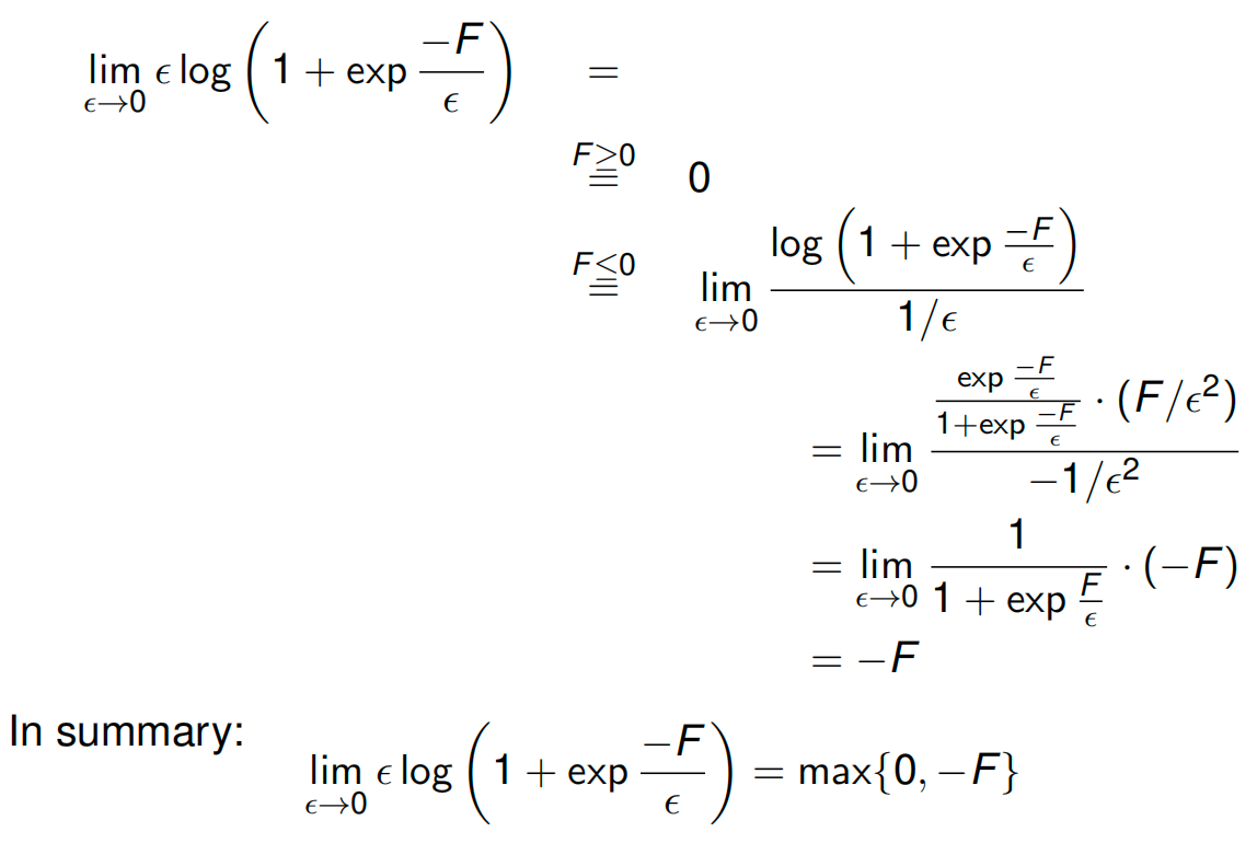
当 $\epsilon \to 0$（温度趋近于 0）时：Log-Sum-Exp 会变成 Max (最大值) 函数。
- 就好比水结冰了，变成了硬邦邦的固体（Hard Max）。
当 $\epsilon = 1$（温度较高）时：它保持平滑，保留了所有可能性的概率分布（Soft Max）。

推导一：变身成 SVM ($\epsilon \to 0$)

让我们看看当温度 $\epsilon$ 变得非常非常小（趋近于 0）时，公式会发生什么。

原理：$\lim_{\epsilon \to 0} \epsilon \ln \sum \exp(\frac{A}{\epsilon}) \approx \max(A)$。
代入公式：

\[\epsilon \ln \sum_{\hat{y}} \exp \frac{L + \mathbf{w}^T \psi}{\epsilon} \quad \xrightarrow{\epsilon \to 0} \quad \max_{\hat{y}} (L(y, \hat{y}) + \mathbf{w}^T \psi(x, \hat{y}))\]
结果：这正好就是 PPT 上半部分写的 Multi-class SVM 的公式（Hinge Loss）！
- 这里的 $L(y, \hat{y})$ 通常就是那个 $1$（Margin），代表如果预测错了要惩罚多少。
- 结论：SVM 其实就是“低温”极限下的逻辑回归。它只关心那个最大的得分（最硬的边界），忽略其他的。

推导二：变身成逻辑回归 ($\epsilon = 1$)

让我们看看当温度 $\epsilon = 1$ 时，公式会发生什么。我们假设这是标准的逻辑回归（没有额外的边界惩罚 $L=0$）。

代入公式：

\[1 \cdot \ln \sum_{\hat{y}} \exp \left( \frac{0 + \mathbf{w}^T \psi(x, \hat{y})}{1} \right) - \mathbf{w}^T \psi(x, y)\]

\[= \ln \left( \sum_{\hat{y}} \exp(\mathbf{w}^T \psi(x, \hat{y})) \right) - \mathbf{w}^T \psi(x, y)\]
这是什么？ 这正是 负对数似然函数 (Negative Log-Likelihood)，也就是逻辑回归用来优化的 交叉熵损失 (Cross-Entropy Loss)。
- 第一项是配分函数（归一化项，$Z$）的对数。
- 第二项是正确类别的得分。
- 结论：逻辑回归是“常温”下的模型。它考虑了所有类别的得分，计算出一个概率分布。

这个公式建立了一个连续的光谱：

光谱的一端 ($\epsilon \to 0$) 是 SVM：它是“硬”的，只在乎最强的那个对手（Support Vectors），计算的是几何间隔。
光谱的另一端 ($\epsilon = 1$) 是 逻辑回归：它是“软”的，考虑全局的概率分布，计算的是概率似然。

一句话概括： SVM 只是逻辑回归在温度冷却到 0 度时的特例。

Binary logistic regression/SVM is convex 凸的

$\phi$

Kernels¶

第一部分：那四个公式是怎么来的？

这四个公式分为两组：训练用的（Dual）*和*预测用的（Prediction）。它们的核心来源都是我们在前面提到的 拉格朗日乘数法。

1. 预测公式 (Prediction with dual variables)¶

\[\mathbf{w}^T \phi(x) = \frac{1}{C} \sum \alpha^{(i)} y^{(i)} \phi(x^{(i)})^T \phi(x)\]

这是什么？ 这是告诉你，一旦模型训练好了，怎么用它来预测新数据。
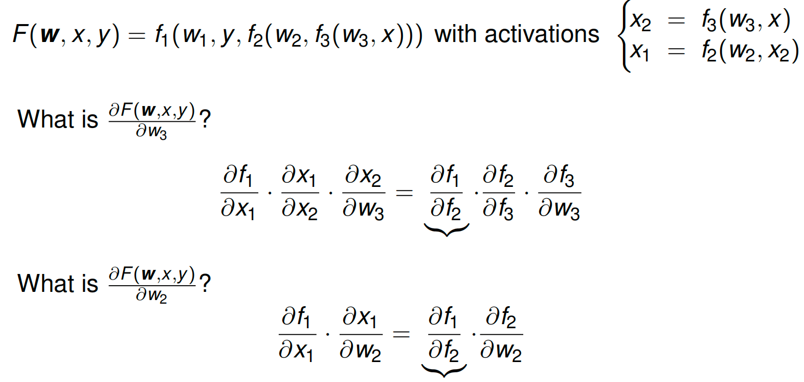
怎么推导的？

还记得在求拉格朗日极值时，我们对 $\mathbf{w}$ 求导并令其为 0 吗？

\[\frac{\partial L}{\partial \mathbf{w}} = 0 \implies \mathbf{w} = \sum \alpha_i y_i \phi(x_i)\]

这个式子被称为 表示定理 (Representer Theorem)。它告诉我们：最佳的权重向量 $\mathbf{w}$ 其实就是所有训练数据点 $\phi(x_i)$ 的线性组合（加权和）。

所以，当我们预测新数据 $\phi(x)$ 时，原本是计算 $\mathbf{w}^T \phi(x)$，现在把 $\mathbf{w}$ 替换掉，就变成了公式里的样子：新数据与所有旧数据的内积的加权和。

2. 对偶问题公式 (Dual of SVM / Logistic)¶

\[\max g(\alpha) := \frac{-1}{2C} \| \sum \dots \|^2 + \sum \alpha\]

这是什么？ 这是训练阶段真正要解的数学题。
怎么推导的？

这就是我们在前几张 PPT 里做的“代回”步骤。

既然我们知道 $\mathbf{w}$ 可以用 $\alpha$（或 $\lambda$）表示，我们就把 $\mathbf{w}$ 的表达式代回到原本的拉格朗日函数 $L$ 中。

这样一来，式子里就没有 $\mathbf{w}$ 了，只剩下对偶变量 $\alpha$ 和数据点之间的内积。
观察点：

你会发现 Logistic Regression 和 SVM 的对偶公式长得非常像。它们都依赖于数据点的内积。区别仅在于约束条件和具体的系数（因为它们的 Loss Function 不同，一个是 Log Loss，一个是 Hinge Loss）。

第二部分：后面的 Kernel 相关是在干什么？

既然我们有了上面的四个公式，数学家们发现了一个惊人的“漏洞”（或者说捷径），这就是 核技巧 (Kernel Trick)。

1. 观察到的现象 (Observation)¶

请看上一张图的四个公式，不管是训练（Dual）还是预测（Prediction），所有的计算都只涉及数据向量之间的内积：

\[\phi(x^{(i)})^T \phi(x^{(j)})\]

也就是说，我们根本不需要单独知道 $\phi(x)$ 长什么样，我们只需要知道两个数据点“乘起来”是多少。

2. 为什么要用 Kernel？¶

假设我们的数据在低维空间不可分，我们需要把它映射到高维空间（比如 100万维）才能分开。

笨办法（不用 Kernel）：
1. 先把 $x$ 映射成 100万维的向量 $\phi(x)$。（计算量爆炸）
2. 再计算这两个 100万维向量的内积。（计算量再次爆炸）
聪明办法（Kernel Trick）：

我们发现有一个函数 $K(x, z)$，它在低维直接算出来的结果，刚好等于那个高维内积的结果。

\[K(x, z) = \phi(x)^T \phi(z)\]

这样我们就可以不用去计算那个复杂的 $\phi(x)$，直接在低维算个 $K$ 就行了。

3. 总结¶

Kernel 是什么？ 它是一个计算捷径。
Advantage (优势)： 不需要显式地构建特征向量 $\phi(x)$。省内存、省时间，还能解决非线性问题。
But (但是)： 不是随便找个函数都能当 Kernel，它必须满足数学条件（Mercer's Theorem），保证它对应某个特征空间里的内积。

一句话总结这两张图的逻辑：

第一张图推导出公式，证明了“只要算出内积就能训练和预测”；第二张图接着说“既然只要内积，那我们就用 Kernel 函数来偷懒，直接算出内积，从而轻松实现高维映射”。

Linear kernel:

Squared exponential (Gaussian) kernel:

Sigmoid kernel:

New kernels:

[!NOTE]

How to extend binary classification to multiple classes?

What are kernels good for?

Deep Nets¶

Deep Learning

AlexNet

Decreasing spatial resolution and the increasing number of channels

Fully connected layer¶

One particular output is influenced by all the other inputs: wx+b

[!NOTE]

What’s an issue with fully connected layers?

Parameter Explosion (Way too many weights)

Loss of Spatial Structure

How to share weights?

we use Convolutional Layers

Convolutions¶

Output width: $$O = \lfloor \frac{W - F + 2P}{S} \rfloor + 1$$

Where:

$W$ = Input Width/Height
$F$ = Filter Size
$S$ = Stride
$P$ = Padding
$\lfloor \dots \rfloor$ means "floor" (round down to the nearest whole number).

The Rule: The depth of the output volume is always exactly equal to the number of filters applied in that layer.

Maximum-/Average pooling¶

After a convolutional layer extracts features (like edges or textures), pooling layers are used to downsample the image. They shrink the spatial dimensions (width and height) while keeping the depth (number of channels) the same. 卷积层提取特征（如边缘或纹理）后，使用池层对图像进行下采样 。它们缩小了空间维度（宽度和高度），同时保持深度（通道数量）不变。

Goal: Reduce the number of parameters and computations in the network, and make the model more robust to slight shifts or distortions in the image (translation invariance). 目标： 减少网络中的参数和计算数量，使模型对图像中的轻微偏移或畸变更具鲁棒性（平移不变性）。
How it works: You slide a window (e.g., $2 \times 2$ with a stride of 2) over the feature map, but instead of calculating a dot product with weights, you just do a simple math operation: 工作原理： 你在特征图上滑动一个窗口（例如 $2 \times 2$ 步幅为 2），但你不是计算带权重的点积，而是做一个简单的数学运算：
- Maximum Pooling: Takes the largest number in the window. This is the most common type. It effectively says, "Did this feature (like a horizontal edge) appear anywhere in this $2 \times 2$ region? If yes, keep the strongest signal and ignore the rest." 最大池 ：取窗口内最大数值。这是最常见的类型。它实际上是在说：“这个特征（比如水平边缘）在这个 $2 \times 2$ 区域里出现过吗？如果是，保留最强的信号，忽略其余。”
- Average Pooling: Takes the mathematical average of the numbers in the window. It smooths the information out. While less common in early layers today, a variation called "Global Average Pooling" is heavily used at the very end of modern networks (like ResNet) to collapse a whole $7 \times 7$ grid into a single number. 平均池： 取窗口内数字的数学平均值。它能让信息变得平滑。虽然在早期层中较少见，但现代网络（如 ResNet）最末端大量使用一种称为“全局平均池”的变体，将整个 $7 \times 7$ 网格压缩为一个数字。

Softmax Layer¶

You actually saw the math for this in your earlier slides on the "Unified Objective Function" / Log-Sum-Exp! 你其实在之前关于“统一目标函数”/对数和-经验的幻灯片中看到过数学计算！

Goal: Convert raw, unnormalized network outputs (called "logits" — which could be anything like $50$, $-12$, or $0.5$) into a valid probability distribution. 目标： 将原始、未归一化的网络输出（称为“logits”——可以是、、或等） $50$ 转换为有效的概率分布 。 $0.5$ $-12$
Where it goes: It is almost always the very last layer of a multi-class classification network. 它去向： 它几乎总是多类别分类网络的最后一层。
The Math: For a given class $i$, the probability is calculated as:

数学： 对于给定的类别 $i$ ，概率计算为：

\[p_i = \frac{e^{z_i}}{\sum_{j} e^{z_j}}\]
- The exponential $e^z$ turns all negative numbers into positives. 指数函数将所有负数 $e^z$ 转换为正数。
- Dividing by the sum of all exponentiated scores ensures that all the final probabilities add up to exactly $1.0$ (or $100\%$). 除以所有指数分数的总和，确保所有最终概率的总和恰好 $1.0$ 为（或 $100\%$ ）。
Why "Soft-max"? It acts like a "Max" function because the exponentiation heavily exaggerates the highest score (the winner takes most of the probability). It is "Soft" because it is differentiable, meaning you can calculate gradients to train the network using backpropagation. 为什么叫“软极限”？ 它的作用类似于“最大”函数，因为指数函数极大地夸大了最高分（获胜者获得大部分概率）。它被称为“软”是因为它可微，意味着你可以计算梯度来训练网络，利用反向传播。

+1

Dropout Layer¶

A dropout layer is a regularization technique. It doesn't extract features or make predictions; its only job is to prevent overfitting (memorizing the training data). dropout 层是一种正则化技术。它不提取特征或做预测;它的唯一任务是防止过拟合 （记忆训练数据）。

How it works: During training, a Dropout layer randomly "turns off" (sets to zero) a certain percentage of neurons in the layer (e.g., $50\%$) for every single batch of data.
Why this is brilliant: * It prevents "co-adaptation." If neurons know their neighbors might randomly disappear, they can't lazily rely on each other. Every neuron is forced to learn useful, independent features. 为什么这很聪明:它防止了“共适应”。如果神经元知道邻居可能会随机消失，就不能懒惰地依赖彼此。每个神经元都被迫学习有用且独立的特征。
- It acts like you are training thousands of slightly different, smaller neural networks at the same time and averaging their results (an ensemble). 它就像你同时训练成千上万个略有不同、规模较小的神经网络，并对它们的结果进行平均（一个集合）。
Note: Dropout is only active during training. When you are deploying the model to make real predictions (inference), you leave all neurons turned on so the model has its full brainpower. 注：退学机制只在训练期间生效。当你部署模型进行真实预测（推理）时，你会保持所有神经元的状态，这样模型才能拥有全部的脑力。

Training¶

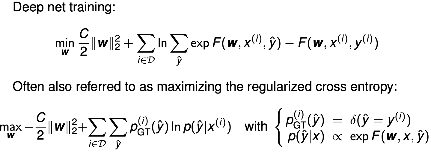
Here is the step-by-step derivation of how the "maximizing the regularized cross entropy" equation turns perfectly into the "Deep net training" equation. 以下是“ 最大化正则化交叉熵” 方程如何完美转化为 “深度网训练” 方程的逐步推导。

Step 1: Simplify the Cross Entropy Sum 步骤1：简化交叉熵和¶

Let's look at the cross-entropy part of the bottom equation:

让我们看看底部方程中的交叉熵部分：

\[\sum_{\hat{y}} p_{\text{GT}}^{(i)}(\hat{y}) \ln p(\hat{y}|x^{(i)})\]

The slide defines the ground truth probability $p_{\text{GT}}^{(i)}(\hat{y})$ as a delta function $\delta(\hat{y} = y^{(i)})$. 幻灯片将基层真实概率定义 $p_{\text{GT}}^{(i)}(\hat{y})$ 为一个δ函数 $\delta(\hat{y} = y^{(i)})$ 。

This means the probability is exactly $1$ when the guess ($\hat{y}$) matches the true label ($y^{(i)}$), and $0$ for every other possible class. 这意味着概率恰好 $1$ 是猜测（y）时 ^ ）匹配真实标签（）， $y^{(i)}$ 并且 $0$ 对所有其他可能的类别都匹配。
Because it is 0 everywhere else, the entire sum over all classes collapses into just one term: the term for the correct class $y^{(i)}$. 由于其他地方都是 0，所有类的和都归纳为一个项：正确的类 $y^{(i)}$ 项。

So, the cross entropy simplifies to:

因此，交叉熵简化为：

\[1 \cdot \ln p(y^{(i)}|x^{(i)})\]

Step 2: Plug in the Softmax Probability 步骤 2：输入 Softmax 概率¶

The slide defines the predicted probability as proportional to the exponential of the network's output: $p(\hat{y}|x) \propto \exp F(\mathbf{w}, x, \hat{y})$.

To make it a true probability that sums to 1, we must divide it by the sum of the exponentials for all possible classes (this is the standard Softmax function):

幻灯片定义了预测概率与网络输出的指数成正比： $p(\hat{y}|x) \propto \exp F(\mathbf{w}, x, \hat{y})$ 。为了使其成为一个真概率且总和为 1，我们必须将其除以所有可能类别的指数函数之和（这就是标准的 Softmax 函数）：

\[p(y^{(i)}|x^{(i)}) = \frac{\exp F(\mathbf{w}, x^{(i)}, y^{(i)})}{\sum_{\hat{y}} \exp F(\mathbf{w}, x^{(i)}, \hat{y})}\]

Step 3: Apply Logarithm Rules 步骤3：应用对数规则¶

Now, we substitute this fraction back into our natural log function from Step 1. Using the rule $\ln(\frac{A}{B}) = \ln(A) - \ln(B)$: 现在，我们将这个分数代回第一步的自然对数函数。使用规则 $\ln(\frac{A}{B}) = \ln(A) - \ln(B)$ ：

\[\ln \left( \frac{\exp F(\mathbf{w}, x^{(i)}, y^{(i)})}{\sum_{\hat{y}} \exp F(\mathbf{w}, x^{(i)}, \hat{y})} \right)\]

\[= \ln(\exp F(\mathbf{w}, x^{(i)}, y^{(i)})) - \ln \left( \sum_{\hat{y}} \exp F(\mathbf{w}, x^{(i)}, \hat{y}) \right)\]

Since the natural log ($\ln$) and exponential ($\exp$) cancel each other out on the first term, we are left with:

由于自然对数（ $\ln$ ）和指数（ $\exp$ ）在第一项相互抵消，我们得到：

\[= F(\mathbf{w}, x^{(i)}, y^{(i)}) - \ln \sum_{\hat{y}} \exp F(\mathbf{w}, x^{(i)}, \hat{y})\]

Step 4: Maximize vs. Minimize 步骤4：最大化与最小化¶

Now, let's substitute our simplified cross entropy back into the full bottom equation:

现在，我们将简化的交叉熵代入完整的底部方程：

\[\max_{\mathbf{w}} \left( - \frac{C}{2}\|\mathbf{w}\|_2^2 + \sum_{i \in \mathcal{D}} \left[ F(\mathbf{w}, x^{(i)}, y^{(i)}) - \ln \sum_{\hat{y}} \exp F(\mathbf{w}, x^{(i)}, \hat{y}) \right] \right)\]

In optimization, maximizing a function is the exact same as minimizing its negative. If we want to change this from a $\max$ problem to a $\min$ problem, we just multiply the entire expression by $-1$. This flips all the signs: 在优化中， 最大化函数与最小化其负值完全相同 。如果我们想把它从一个 $\max$ 问题变为 $\min$ 一个问题，我们只需将整个表达式乘以 $-1$ 。这颠倒了所有迹象：

\[\min_{\mathbf{w}} \left( + \frac{C}{2}\|\mathbf{w}\|_2^2 + \sum_{i \in \mathcal{D}} \left[ - F(\mathbf{w}, x^{(i)}, y^{(i)}) + \ln \sum_{\hat{y}} \exp F(\mathbf{w}, x^{(i)}, \hat{y}) \right] \right)\]

Rearrange the terms inside the bracket, and you get exactly the "Deep net training" equation at the top of the slide. 把括号内的术语重新排列 ，你就能得到幻灯片顶部的“深网训练”公式。

Summary 摘要¶

The top equation is just the negative log-likelihood (cross-entropy) written out in its raw algebraic form. Maximizing the probability of the correct answers is mathematically identical to minimizing the error (loss) function. 顶部方程就是以原始代数形式写出的负对数似然（交叉熵）。最大化正确答案的概率在数学上与最小化误差（损失）函数是相同的。

What is C? Weight decay (aka regularization constant)

Loss function¶

CrossEntropyLoss: $loss(x, class) = -\frac{log(exp(x[class])}{ (\sum_j exp(x[j])))} = -x[class] + log(\sum_j exp(x[j]))$

NLLLoss: $loss(x, class) = -x[class]$

MSELoss: $loss(x, y) = 1/n \sum_i |x_i - y_i|^2$

BCELoss: $loss(o,t)=-1/n \sum_i i(t[i]*log(o[i])+(1-t[i])*log(1-o[i]))$

o: probability model

BCEWithLogitsLoss: $loss(o,t)=-1/n\sum_i(t[i]*log(sigmoid(o[i])) +(1-t[i])*log(1-sigmoid(o[i])))$

o:

L1Loss

KLDivLoss

class Net(nn.Module):
def __init__(self):
  super(Net, self).__init__()
  self.conv1 = nn.Conv2d(1, 6, 5)
  self.conv2 = nn.Conv2d(6, 16, 5)
  self.fc1 = nn.Linear(16 * 5 * 5, 120)
  # 16 chanels, 5*5 spatial space
  self.fc2 = nn.Linear(120, 84)
  self.fc3 = nn.Linear(84, 10)
def forward(self, x):
  x = F.max_pool2d(F.relu(self.conv1(x)), (2, 2))
  x = F.max_pool2d(F.relu(self.conv2(x)), 2)
  x = x.view(-1, self.num_flat_features(x))
  x = F.relu(self.fc1(x))
  x = F.relu(self.fc2(x))
  x = self.fc3(x)
  return x

What are the input dimensions?

What are deep nets?

How do deep nets relate do SVMs and logistic regression

What components of deep nets do you know?

What algorithms are used to train deep nets?

forward and backward pass¶

Forward: x2->f2

Backpropagation¶

Repeated use of chain rule for efficient computation of all gradients

Initilization

Remark

Popular architectures¶

LeNet

AlexNet

VGG (16/19 layers, mostly 3x3 convolutions)

GoogLeNet (inception module)

ResNet (residual connections)

What are deep nets?

How do deep nets relate do SVMs and logistic regression

What is back-propagation in deep nets?

What components of deep nets do you know?

What algorithms are used to train deep nets?

Structured Prediction (exhaustive search, dynamic programming)¶

structure/correlations are useful

Predictions from neighboring pixel are useful

k-Means Clustering¶

Cost function

What is the cost function for kMeans?

What are the steps of the kMeans algorithm?

What are the guarantees of the kMeans algorithm?

Gaussian Mixture Models¶

What is the maximum likelihood solution of fitting the mean and variance of a Gaussian?

Why do we consider mixtures of Gaussians?

How do we find the means, variances and responsibilities of the Gaussian mixture model?

Expectation Maximization/Majorize-Minimize/Concave-convex procedure¶

评论区~

有用的话请给我个赞和 star =>